­N-Dimensional Dictionary Learning for Hyperspectral Scanning (Transmission) Electron Microscopy

Session

Poster Session Three

Authors

Jack Wells (1), Daniel Nicholls (1), Alex Robinson (1), Amir Moshtaghpour (1), Jony Castagna (1), Yalin Zheng (1), Nigel Browning (1, 2, 3)

Affiliations

1. University of Liverpool
2. Pacific Northwest National Laboratory
3. Sivananthan Laboratories

Keywords

4D-STEM

Bayesian

Dictionary Learning

Inpainting

Hyperspectral

Ptychography

EDX

Abstract text

Over the last few years, methods in Dictionary Learning and/or Image Inpainting have been successfully applied to many different forms of Electron Microscopy (EM) data. [2, 6]. In the context of these methods, a dictionary of atoms can be used to sparsely represent each overlapping patch as a linear combination of a small number of dictionary elements and their corresponding coefficients. The choice of dictionary atoms can be learned from fully-sampled data using traditional techniques such as K-SVD [1] or directly from subsampled data using Bayesian methods such as Beta-Process Factor Analysis (BPFA) [2], and the resulting sparse representations can be used for tasks such as compression [3], inpaintingsubsampled reconstruction [2], denoising [4], and image classification [5]. Typically, this target “image” data would be 2-dimensional (2D), such as Z-contrast images from a Scanning Transmission Electron Microscope (STEM), or in some cases 3-dimensional (3D), such as RGB images, successive 2D layers of a 3D volume e.g. cryo-FIB, or Energy-dispersive X-ray spectroscopy (EDS) maps which use the third dimension for discretised spectral information. In most historical approaches, for an “image” of shape M = (M₀ x M₁ x M₂), the dictionaries used represent a set of (vectorised) elements with a patch shape B defined only in the first two dimensions – that is, patches with a height (B₀ << M₀) and width (B₁ << M₂), where the size of the patch in the third dimension spans the entire shape of the target data cube. For the simple cases of 2D/Greyscale images (M₂ =1)  and RGB images (M₂ = 3), this is an obvious approach; In fact, in many cases, the patch shape B is defined by a single integer value b (b = B₀ = B₁) such as b=10, where patches take the shape of B = (10 x 10 x M₂).

Data Type	Shape	Dimensionality
Greyscale Video e.g. (multi-frame) STEM BF/ABF/ADF/HAADF data	3D	Height , Width , Frames
RGB Video e.g. (multi-frame) combinatorial acquisition / colourised data	4D	Height, Width, Channels, Frames
Hyperspectral Video e.g. (multi-frame) EDS/EELS data	4D	Height, Width, Spectrum, Frames
Series of Diffraction Patterns e.g. 4D-STEM/Ptychography, EBSD data	4D	x, y, Height, Width

Table 1: Examples of higher-dimensional EM data types / multi-frame targets and their corresponding dimensionality.

However, there are many examples of higher-dimensional EM data, and more complex tasks such as real-time (frame-by-frame) reconstructions (see Table 1) that would benefit from variable patch shapes in higher dimensions. For the case of multi-frame targets such as greyscale and RGB video, this could represent dictionary elements trained with a higher-dimensional patch shape spanning a few (or more) frames of the video, i.e. capturing representative signal patterns for the change in pixel values with respect to time in addition to the spatial dimensions, or conversely, training/inpainting with a single-channel dictionary for 2D patches across each layer of a multi-channel (e.g. RGB) data source. For hyperspectral data cubes, it may represent the generation/use of a dictionary spanning an arbitrary  “steps”  across a discretised spectrum, or a method of frame-interpolation for data cubes subsampled in the fourth (time) dimension. This much more varied patch shape also allows for further, more complex scenarios, such as dictionary transfer between a 2D high-SNR source such as a Back-Scattered Electron (BSE) image and the low-SNR constituent “layers” of a 3D Energy-dispersive X-ray spectroscopy (EDS) map, improving the quality of reconstruction results [6] as well as reducing the complexity (and thus time-to-solution) of the dictionary learning/inpainting task. The extension of dictionary learning and/or image inpainting algorithms into this N-dimensional context, especially with the goal of performing on batches of n_batch arbitrarily indexed (e.g. programmatically selected) patches/signals from the target data cube necessitates the development of efficient implementations of signal extraction as well as reconstruction/recombination (beyond the capabilities of standard “unwrap”/ “wrap” methods respectively in most computational libraries); However, with a sufficiently optimised implementation, it can provide a significant improvement to the speed of real-time reconstructions on large datasets, a boost to reconstruction quality for low-SNR data, and may even enable completely new uses of a trained dictionary, such as dictionary transfer between “layers”, frame-interpolation, and  a combination of detector and/or probe subsampling for 4D-STEM/Ptychography. [7]

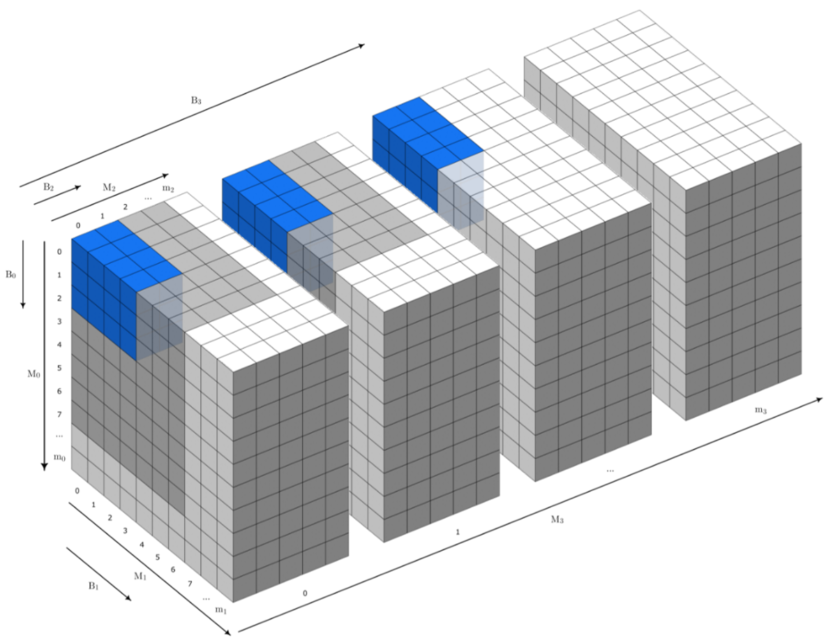
Figure 1: An illustration of a 4D patch of shape B = (B₀ x B₁ x B₂ x B₃) within a 4D target data source of shape M = (M₀ x M₁ x M₂ x M₃) where (for each dimension i). Lower case variables m_i denote the last (zero-based) index in the dimension. Cells shown in grey signify valid patch indexes (indexed by the location of the first contained cell) for the given patch shape (shown in blue)

References

[1] M. Aharon et al., IEEE Transactions on Signal Processing, 54 (2006).

[2] D. Nicholls et al., Ultramicroscopy, 233 (2022).

[3] H. Wang, et al., IEEE International Conference on Image Processing, pp. 3235-3239 (2017).

[4] W. Dong et al., CVPR 2011, pp. 457-464 (2011)

[5] T. H. Vu et al., IEEE Transactions on Medical Imaging, 35 (2016)

[6] D. Nicholls et al., ICASSP 2023 (2023).

[7] The authors acknowledge funding from ESPRC and Sivananthan Laboratories, IL USA.